Circles: Good and Fast, Part 1
After making the Series002 postcards I realized that I was going to have to optimize some speeds to get more ambitious plots done in a reasonable time. For those plots, which were all straight lines, the front of a sheet of 4 postcards (the art side), took about 15 minutes to plot. Not bad. The back, which was basically all text (maybe too much text), took over an hour to plot. This is too slow.
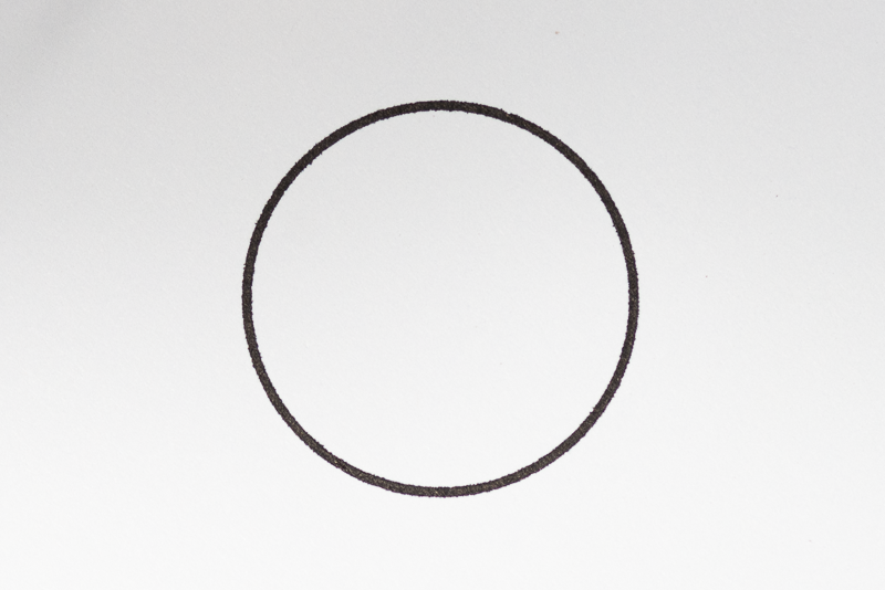
Now, you might think I should start by making text plot faster. You might be right about that. But I want a laboratory to study first. I happen to know that when I first added my circle drawing code for the Series001 postcards, I just picked a step size that I knew would be good enough to make nice round circles (see above, for example). It’s a perfect thing to optimize.
Note: Circles, and curves, are not in fact smooth curves when plotted. They are many small straight lines. A circle is drawn as a regular polygon with many (many-many) sides.
Maybe next I’ll do squares, or regular polygons with O(10) sides or fewer. I think there will be plenty to learn with this subject.
The Situation
Lets start with some basics. A) I just got this plotter a month ago. I love it. But, B) I have no real idea what I am doing. C) I want to do everything myself, for reasons, so I am only doing things via the python API directly in interactive mode. So, some of these first assumptions may be wrong to begin with. But this is about exploring. These are the initial settings:
speed_pendown = 20I don’t know why I set the pen down speed to 20. What even are the units? According to the API docs, it’s expressed as a percentage of the maximum travel speed. What is the maximum travel speed? And the default is 25, so my value is only 5% less than the default.
For future reference, here are all the values in the AxiDraw.options attribute:
{'ids': [],
'selected_nodes': [],
'speed_pendown': 20,
'speed_penup': 75,
'accel': 75,
'pen_pos_down': 30,
'pen_pos_up': 60,
'pen_rate_lower': 50,
'pen_rate_raise': 75,
'pen_delay_down': 0,
'pen_delay_up': 0,
'no_rotate': False,
'const_speed': False,
'report_time': False,
'page_delay': 15,
'preview': False,
'rendering': 3,
'model': 2,
'port': None,
'setup_type': 'align',
'resume_type': 'plot',
'auto_rotate': True,
'reordering': 0,
'resolution': 1,
'mode': 'interactive',
'manual_cmd': 'fw_version',
'walk_dist': 1,
'layer': 1,
'copies': 1,
'port_config': 0,
'units': 0}
Below is also a listing of my circle drawing code.
import math
from loguru import logger
from pyaxidraw import axidraw

axi = axidraw.AxiDraw()

def circle_edge_pt(x_coord, y_coord, radius, theta):
    """Get a point along the perimeter of a circle."""
    return (x_coord + radius * math.sin(theta),
            y_coord + radius * math.cos(theta))

def draw_arc(axi,
             x_coord,
             y_coord,
             radius,
             theta0=0,
             total_theta=2 * math.pi,
             step_distance=0.01):
    """Draw a perfect circle."""
    # pylint: disable=too-many-arguments
    logger.trace(
        f"Drawing arc at {x_coord}, {y_coord}, {theta0} : {total_theta}.")
    step_size = step_distance / radius
    axi.moveto(
        *circle_edge_pt(x_coord, y_coord, radius, theta0))
    for i in range(int(total_theta / step_size) + 1):
        point = CircleTools.circle_edge_pt(x_coord, y_coord, radius,
                                           (theta0 + (i + 1) * step_size))
        axi.lineto(*point)
Some things to say about this code. The shooting step size (listed as step_distance above) is 0.01 inches, or 0.254 mm.
Measuring Current Speed
With the above in hand, lets measure how much time it takes to draw some circles. I’ve never really measured this before in python, so I’m going to search for some guidance. This article looks pretty promising. Just doing the basics, using the time.perf_counter function to do some tic/toc style measuring looks like it will get us started.
import math
import time

radius = 0.5  # inches.
tic = time.perf_counter()
draw_arc(axi, 2, 2, radius)
toc = time.perf_counter()
print(f"time to draw a {2 * radius} inch "
      f"diameter circle was {toc - tic:0.1f} seconds")
print(f"total line length was {2 * radius * math.pi:0.2f} inches")
time to draw a 1.0 inch diameter circle was 23.8 seconds
total line length was 3.14 inchesI measured a value of 23.8 seconds to draw a 3.14 inch long line, or 0.13 inches / second (3.3 mm/s). This is rather slow. I think we can do a lot better. Incidentally, to draw that circle, the code above made 1257 individual moves. That’s a lot of moves. But it is a very nice circle.
My hope is that I can get a circle basically as good but in a fraction of the time. I’m not sure what is achievable, but I set an arbitrary goal of one tenth of the original time, or 2.3 seconds. My immediate reaction is that this is wildly ambitious. First, let’s make a plan, and always re-evaluate if this is reasonable.
The plan
OK, so I had a moment to think and I realized that there is more to drawing circles than just moving the pen around. Ink must flow out of the pen as well. Maybe we can draw the circle in 2.3 seconds, but with one pen we’ll get a nice solid line and another will give something much less nice. But anyway, here is what we’re going to do:
- Increase the step shooting distance (the step size)
- Change the pen down speed (how fast it draws the line)
- The end point may in fact be too far, so examine that too (don’t draw more circle than necessary)
- Verify that the circles are still good (that is, still circular)
- Circle back, ahem, to the issue of pen down speed to address the ink flow
So there it is, that’s the plan. Let’s do it.
Step 1: Increase the shooting distance
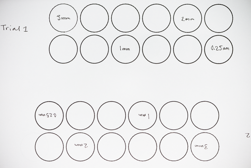
So this is a simple one. The basic idea is to draw circles varying the step size and observe a few things. Here is the recipe.
- Draw 1 inch diameter circles, starting with 3 mm steps, down to 0.25 mm.
- Measure how long it takes to draw each circle, and the total line length.
- View the circles closely to see how well they appear circular.
Below is an SVG of the file that will be drawn. Later down, there is a picture of the plotted page.

I plotted the file twice and collected the data. The result is reproduced below.
Trial 1:
| shooting distance (mm) | run time (s) | total distance (mm) |
|---|---|---|
| 3.00 | 4.5 | 162.00 |
| 2.75 | 9.3 | 165.00 |
| 2.50 | 9.0 | 160.00 |
| 2.25 | 9.2 | 162.00 |
| 2.00 | 9.1 | 160.00 |
| 1.75 | 9.5 | 161.00 |
| 1.50 | 11.0 | 162.00 |
| 1.25 | 11.0 | 160.00 |
| 1.00 | 12.3 | 160.00 |
| 0.75 | 14.1 | 160.50 |
| 0.50 | 17.1 | 160.00 |
| 0.25 | 23.8 | 160.00 |
Trial 2:
| shooting distance (mm) | run time (s) | total distance (mm) |
|---|---|---|
| 3.00 | 4.5 | 162.00 |
| 2.75 | 9.3 | 165.00 |
| 2.50 | 9.0 | 160.00 |
| 2.25 | 9.1 | 162.00 |
| 2.00 | 9.0 | 160.00 |
| 1.75 | 9.5 | 161.00 |
| 1.50 | 11.0 | 162.00 |
| 1.25 | 11.0 | 160.00 |
| 1.00 | 12.3 | 160.00 |
| 0.75 | 14.1 | 160.50 |
| 0.50 | 17.1 | 160.00 |
| 0.25 | 23.8 | 160.00 |
It’s easier to see in graphical form.
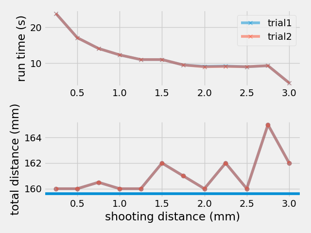
- The two trials are basically identical, in terms of time. That repeatability is really nice to see.
- The distance is going to be identical since that’s just a mathematical accumulation, not a record of the travel distance of the physical device.
- It’s a pretty smooth reduction in time as the step size increases, but it plateau’s by about 1 mm. I had (naively) expected it to be linear.
- There is a dramatic fall off between 2.75 mm and 3 mm step size. This is really unexpected, it’s basically 1/2 the time.
- A note about the overshoot. As shown in the bottom plot, all the circles overshoot the mark. This is expected since (but not desirable) the loop that draws the circles doesn’t take care on the last step to precisely end at the desired length.
- A last comment about the code: it doesn’t guard against a negative step size.
I’ll end this part with the list of questions that I have, and they’re likely to be the topics in the next post in the series.
- Why is the “time to plot” non-linear? And why does it drop off the cliff at 3 mm?
- Observationally with the real output, about 1 mm is the best step size. The pre-render it looks like we could have done bigger. What is going on?
- What is a theoretical expected step size? How can we motivate a good choice?
And of course continue with the plan. See you next time.